The OpenStreetMap community provides free and open geographic data! You may wonder how to use this data in R and that is what we’ll cover in this post.

Which packages?

We’ll use the package osmdata to get access to the OpenStreetMap (OSM) data. sf gives us the basic functions to work with geographic data and we use dplyr and tidyr for data manipulation. ggplot2 and geomtextpath will be used for the visualization.

require(sf)
require(osmdata)
require(dplyr)
require(tidyr)
require(ggplot2)
require(geomtextpath)

Load the data

First we have to set the extent of which we want to get the data. I chose the district La Guillotiere-Sud in Lyon.

# Create bounding box of desired extent
extent <- tibble(
  lon = c(4.833075520540814, 4.851088606828741),
  lat = c(45.747993822856955, 45.755631222240936)  
)

bbox <- extent %>% 
  st_as_sf(coords = c("lon", "lat"), crs = "WGS84") %>% 
  st_bbox()

Next we will use the function opq to build a query to the OSM database with the information of our extent bbox. With add_osm_feature() we can download different features from OSM, in our case these are “building”, “highway” and “waterway”. Here you can see the full list of possibilities. osmdata_sf will return the desired feature as an sf object. We will intersect the output again because the extent of the received data is slightly bigger.

# Get polygons of the feature building
df_build <- opq(bbox = bbox) |> 
    add_osm_feature(key = "building", value_exact = FALSE) |> 
    osmdata_sf()  

df_build_poly <- df_build$osm_polygons |> 
  select(geometry, building, public_transport) # get all buildings and information about usage as public transport

# Get lines of the feature highway
df_highw <- opq(bbox = bbox) |> 
    add_osm_feature(key = "highway", value_exact = FALSE) |> 
    osmdata_sf()  

df_streets <- df_highw$osm_lines |> 
  select(geometry, name) |> 
  st_intersection(st_as_sfc(bbox)) |> 
  na.omit() |> # get rid of small features with no names
  group_by(name) |> 
  # Here we summarise the geometries of the streets, this is necessary to plot the names of the streets later
  summarise(geometry = st_union(geometry)) |> 
  ungroup()

# Get lines of the feature waterway
df_waterw <- opq(bbox = bbox) |> 
    add_osm_feature(key = "waterway", value_exact = FALSE) |> 
    osmdata_sf() 

df_river <- df_waterw$osm_lines |> 
  select(geometry, name)|> 
  st_intersection(st_as_sfc(bbox))

Note: We actually do not only get the polygons or lines but also the features which are points or other geometries.

names(df_build)

[1] "bbox"              "overpass_call"     "meta"             
[4] "osm_points"        "osm_lines"         "osm_polygons"     
[7] "osm_multilines"    "osm_multipolygons"

Plot the data

Now we just have to plot our data. I use the function geom_textsf() from the package geomtextpath to add labels to the river and the streets. Note that you have to declare that you used the data from OSM, see here for more informations. In the case of buildings, we differentiate between whether they are public transportation or not. This is because the subway stations are also part of buildings. We put them in a lighter gray under the streets!

ggplot() +
  geom_textsf(data = df_river,
          aes(geometry = geometry,
              label = name),
          text_smoothing = 99.5,
          linecolour = "#8888B3",
          linewidth = 20,
          color = "black", 
          alpha = 0.8, 
          size = 3, 
          hjust = 0.01,
          vjust = -0.01) +
  geom_sf(data = df_build_poly |> filter(!is.na(public_transport)),
          aes(geometry = geometry),
          fill = "grey90") +
  geom_textsf(data = df_streets,
          aes(geometry = geometry,
              label = name),
          color = "black",
          linecolor = "black",
          alpha = 1,
          fontface = 3,
          size = 1.5,
          remove_long = T) +
  geom_sf(data = df_build_poly |> filter(is.na(public_transport)),
          aes(geometry = geometry),
          fill = "grey50") +
  theme_void() +
  labs(title = "LYON - LA GUILLOTIÈRE-SUD",
       caption = "Data from OpenStreetMap") +
  theme(plot.title = element_text(face = "bold"),
        plot.caption = element_text(size = 7))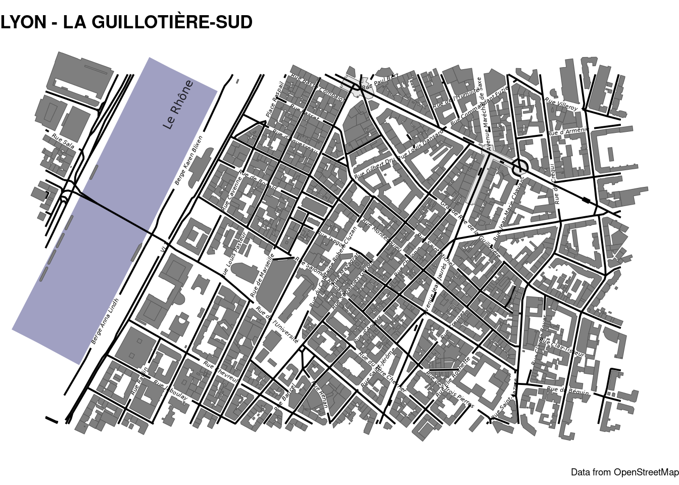

To be honest, the street names are not really readable and a bit confusing in this map. So lets do it again without!

ggplot() +
  geom_textsf(data = df_river,
          aes(geometry = geometry,
              label = name),
          text_smoothing = 99.5,
          linecolour = "#8888B3",
          linewidth = 20,
          color = "black", 
          alpha = 0.8, 
          size = 3, 
          hjust = 0.01,
          vjust = -0.01) +
  geom_sf(data = df_build_poly |> filter(!is.na(public_transport)),
          aes(geometry = geometry),
          fill = "grey90") +
  geom_sf(data = df_streets,
          aes(geometry = geometry),
          color = "black",
          linewidth = 0.8
          ) +
  geom_sf(data = df_build_poly |> filter(is.na(public_transport)),
          aes(geometry = geometry),
          fill = "grey50") +
  theme_void() +
  labs(title = "LYON - LA GUILLOTIÈRE-SUD",
       caption = "Data from OpenStreetMap") +
  theme(plot.title = element_text(face = "bold"),
        plot.caption = element_text(size = 7))

Further ressources

The package osmdata: https://github.com/ropensci/osmdata
The package osmectract: https://github.com/ropensci/osmextract/
Website of OSM: https://www.openstreetmap.org/